SaTScan is a powerful stand-alone software program that runs spation-temporal scan statistics. It is carefully optimized and contains many tricks to reduce the computational burden of the approach, which is doubly computationaly intensive. First, scanning itself can be costly, particularly in spatio-temporal settings. However, even more difficult, testing involves resampling (Monte Carlo hypothesis testing). For these reasons, it is not worthwhile to attempt replicating SaTScan. In addition, while SaTScan is not open source, it is distributed free of charge.

However, use of SaTScan can be cumbersome. There are two means of access: a GUI, and a batch file. The GUI allows complete control, but precludes automated or repeated operation. The batch file allows this, but may be difficult to integrate into other analyses. The rsatscan package contains a set of functions and defines a class and methods to make it easy to work with SaTScan from R. This should allow easy automation and integration.

The functions in the package can be grouped into three sets: SaTScan parameter functions that set parameters for SaTScan or write them in a file to the OS; write functions that write R data frames to the OS in SaTScan-readable formats; and the satscan() function, which calls out into the OS, runs SaTScan, and returns a satscan class object. Successful use of the package requires a fairly precise understanding of the SaTScan parameter file, for which users are referred to the SaTScan manual.

Space-Time Permutation example: NYC fever data

The New York City fever data, which are distributed with SaTScan, are also included with the package.

head(NYCfevercas)

##     zip cases       date
## 1 11229     1 2001/11/22
## 2 11208     1 2001/11/13
## 3 11208     1 2001/11/24
## 4 11212     1  2001/11/3
## 5 11374     1 2001/11/10
## 6 10452     1 2001/11/20

head(NYCfevergeo)

##     zip      lat      long
## 1 10001 40.75037 -73.99674
## 2 10002 40.72199 -73.99000
## 3 10003 40.73097 -73.98841
## 4 10004 40.68834 -74.02002
## 5 10005 40.70550 -74.00816
## 6 10006 40.70754 -74.01292

For good style, an analysis would begin by resetting the paremeter file:

invisible(ss.options(reset=TRUE))

Then, one would change parameters as desired. This can be done in as many or few steps as you like; the previous state of the parameter set is retained, as in par() or options(). Here, the parameters used in the example from the SaTScan manual are replicated:

ss.options(list(CaseFile="NYCfever.cas", PrecisionCaseTimes=3))
ss.options(c("StartDate=2001/11/1","EndDate=2001/11/24"))
ss.options(list(CoordinatesFile="NYCfever.geo", AnalysisType=4, ModelType=2, TimeAggregationUnits=3))
ss.options(list(UseDistanceFromCenterOption="y", MaxSpatialSizeInDistanceFromCenter=3, NonCompactnessPenalty=0))
ss.options(list(MaxTemporalSizeInterpretation=1, MaxTemporalSize=7))
ss.options(list(ProspectiveStartDate="2001/11/24", ReportGiniClusters="n", LogRunToHistoryFile="n"))

Note that the second call to ss.options() uses the character vector format, while the others use the list format; either works.

It might be reasonable at this point to check what the parameter file looks like:

head(ss.options(),3)

## [1] "[Input]"               ";case data filename"   "CaseFile=NYCfever.cas"

Then, we write the parameter file, the case file, and the geometry file to some writeable location in the OS, using the functions in package. These ensure that SaTScan-readable formats are used.

td = tempdir()
write.ss.prm(td, "NYCfever")
write.cas(NYCfevercas, td, "NYCfever")
write.geo(NYCfevergeo, td, "NYCfever")

The write.??? functions append the appropriate file extensions to the files they save into the OS.

Then we’re ready to run SaTScan. The default locations in the function correspond to the location of the executable on my disk, so those or not specified here.

NYCfever = satscan(td, "NYCfever")

## Loading required package: foreign
## Loading required package: rgdal
## Loading required package: sp
## rgdal: version: 0.9-1, (SVN revision 518)
## Geospatial Data Abstraction Library extensions to R successfully loaded
## Loaded GDAL runtime: GDAL 1.11.1, released 2014/09/24
## Path to GDAL shared files: C:/Users/KK/Documents/R/win-library/3.1/rgdal/gdal
## GDAL does not use iconv for recoding strings.
## Loaded PROJ.4 runtime: Rel. 4.8.0, 6 March 2012, [PJ_VERSION: 480]
## Path to PROJ.4 shared files: C:/Users/KK/Documents/R/win-library/3.1/rgdal/proj

The rsatscan package provides a summary method for satscan objects.

summary(NYCfever)

## Prospective Space-Time analysis 
## scanning for clusters with high rates 
## using the Space-Time Permutation model. 
##  
## Study period.......................: 2001/11/1 to 2001/11/24 
## Number of locations................: 192 
## Total number of cases..............: 194 
## _______________________________________________________________________________________________ 
##  
## 
## There were 3 clusters identified.
## There were 0 clusters with p < .05.

The satscan object has a slot for each possible output file that SaTScan creates, and contains whatever output files your call happened to generate.

summary.default(NYCfever)

##            Length Class                    Mode     
## main       138    -none-                   character
## col         15    data.frame               list     
## rr           1    -none-                   logical  
## gis         11    data.frame               list     
## llr          1    data.frame               list     
## sci          6    data.frame               list     
## shapeclust   3    SpatialPolygonsDataFrame S4       
## prm        264    -none-                   character

If SaTScan generated a shapefile, satscan() reads it, by way of the rgdal function readOGR(), if it’s available, into a class defined in the sp package. You can use the plot methods defined in the sp package to plot it, or use one of the many packages that builds on the sp package for further processing.

# sp::plot(NYCfever$shapeclust)

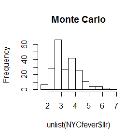
It might be interesting to examine the scan statistics from the Monte Carlo steps.

hist(unlist(NYCfever$llr), main="Monte Carlo")

# Let's draw a line for the clusters in the observed data
abline(v=NYCfever$col[,c("TEST_STAT")], col = "red")

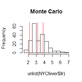
This shows why none of the observed clusters had small p=values.

Poisson spatio-temporal example: New Mexico brain tumor data

This is another data set included with SaTScan. It differs from the NYC fever examle in that denominators are available; these are porvided in a population file. The analysis uses the Poisson model rather than the Spatio-temporal permutation.

write.cas(NMcas, td,"NM")
write.geo(NMgeo, td,"NM")
write.pop(NMpop, td,"NM")

Again, replicating the examples from the SaTScan user guide, we set up and then write the parameter file, then run SaTScan.

invisible(ss.options(reset=TRUE))
ss.options(list(CaseFile="NM.cas",StartDate="1973/1/1",EndDate="1991/12/31", 
                PopulationFile="NM.pop",
                CoordinatesFile="NM.geo", CoordinatesType=0, AnalysisType=3))
ss.options(c("NonCompactnessPenalty=0", "ReportGiniClusters=n", "LogRunToHistoryFile=n"))

write.ss.prm(td,"testnm")
testnm = satscan(td,"testnm")

Note that the parameter file need not have the same name as the case and other input files, which also need not share a name, though it may be helpful in keeping things organized later.

summary(testnm)

## Retrospective Space-Time analysis 
## scanning for clusters with high rates 
## using the Discrete Poisson model. 
##  
## Study period.......................: 1973/1/1 to 1991/12/31 
## Number of locations................: 32 
## Total population...................: 1344288 
## Total number of cases..............: 1175 
## Annual cases / 100000..............: 4.6 
## 
## There were 3 clusters identified.
## There were 1 clusters with p < .05.

One of the elements of a satscan class object is the parameter set which was used to call SaTScan. This may be useful, later.

head(testnm$prm,10)

##  [1] "[Input]"                                                    
##  [2] ";case data filename"                                        
##  [3] "CaseFile=NM.cas"                                            
##  [4] ";control data filename"                                     
##  [5] "ControlFile="                                               
##  [6] ";time precision (0=None, 1=Year, 2=Month, 3=Day, 4=Generic)"
##  [7] "PrecisionCaseTimes=1"                                       
##  [8] ";study period start date (YYYY/MM/DD)"                      
##  [9] "StartDate=1973/1/1"                                         
## [10] ";study period end date (YYYY/MM/DD)"

rsatscan

Ken Kleinman

2015-02-19

Space-Time Permutation example: NYC fever data

Poisson spatio-temporal example: New Mexico brain tumor data

Bernoulli purely spatial example: North Humberside leukemia and lymphoma